31 December 2025

Chest X-Ray Classification with DINOv3

Training a Neural Network to Spot Disease

100,000 X-Rays and a simple disease classifier based on Meta’s DINOv3.

If you’re into chest X-rays and neural networks, this blog post is for you.

Will AI Replace Radiologists?

As a physician who codes, I get this question a lot. The honest answer: I don’t think so. But who knows? Rather than speculate, I decided to dip my toes.

I recently trained a NSFW classifier. Chest X-rays seemed like another interesting challenge: Simple inputs, lots of public data and the diseases are (in theory) visually distinct.

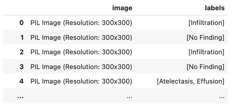
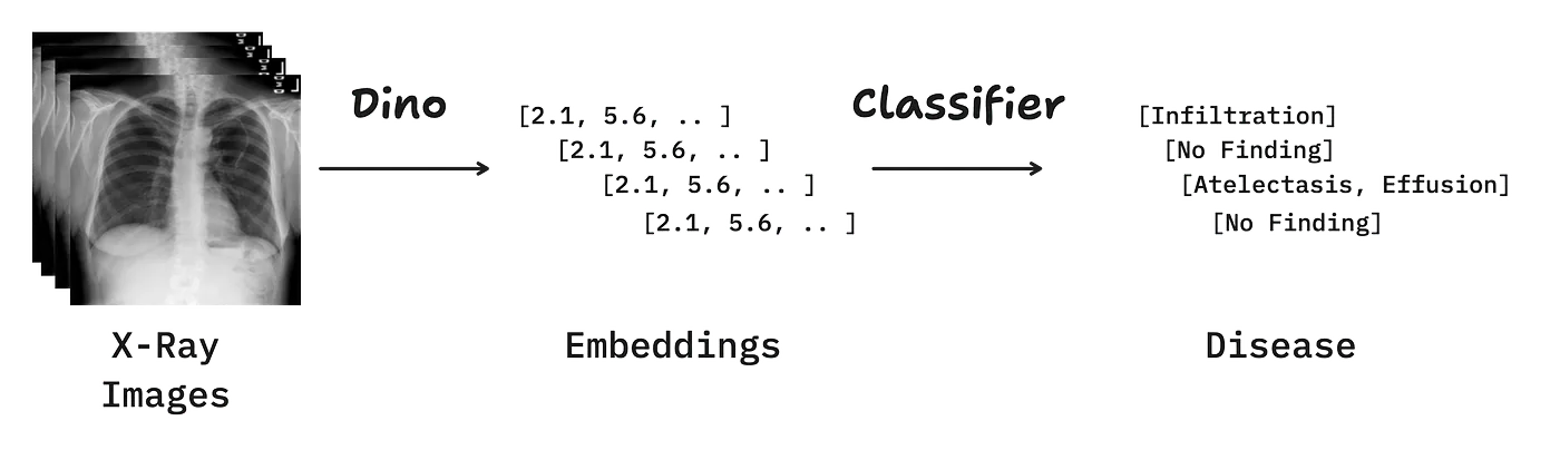
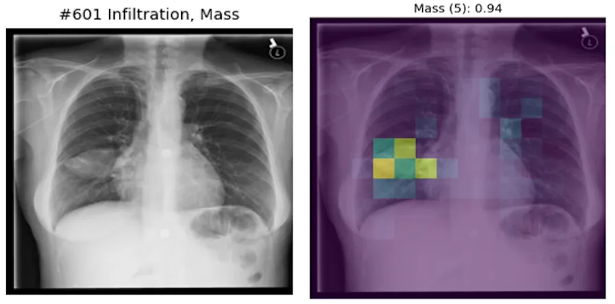
The Dataset. alkzar90/NIH-Chest-X-ray-dataset

The results knocked me off my chair. DINOv3, a tiny vision encoder with 21M parameters, and a simple linear layer learned to localize pathologies from “just” text-labeled images.

Input image and labels on the left. Visualized attention scores of DINOv3-based classifier on the right. — Input image and labels on the **left**. Visualized attention scores of DINOv3-based classifier on the **right**.

The AI didn’t work perfectly. It failed in unexpected ways. A closer look reveals flaws in my thinking about the problem and (maybe) the dataset.

Let’s dive in.

Dataset

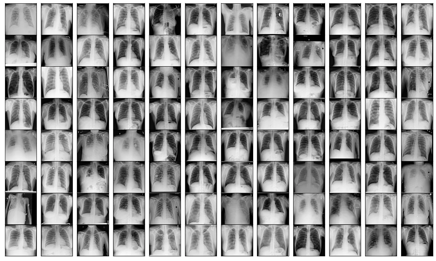
More than 100,000 chest X-rays, published 2017, pulled from HuggingFace.

112,120 frontal-view X-ray images of 30,805 unique patients with the text-mined fourteen disease image labels (where each image can have multi-labels), mined from the associated radiological reports using natural language processing.

Fourteen common thoracic pathologies include Atelectasis, Consolidation, Infiltration, Pneumothorax, Edema, Emphysema, Fibrosis, Effusion, Pneumonia, Pleural_thickening, Cardiomegaly, Nodule, Mass and Hernia, which is an extension of the 8 common disease patterns listed in our CVPR2017 paper.

The text-mined disease labels are expected to have accuracy >90%.

Each image is tagged with at least one label like pneumonia, pleural effusion etc. Some are tagged with two labels, others with even three etc.

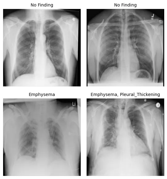
My initial approach of training a classifier to predict all the pathologies in an image failed.

Problem Incoming

The majority of the images are normal (“No finding”), without any pathology.

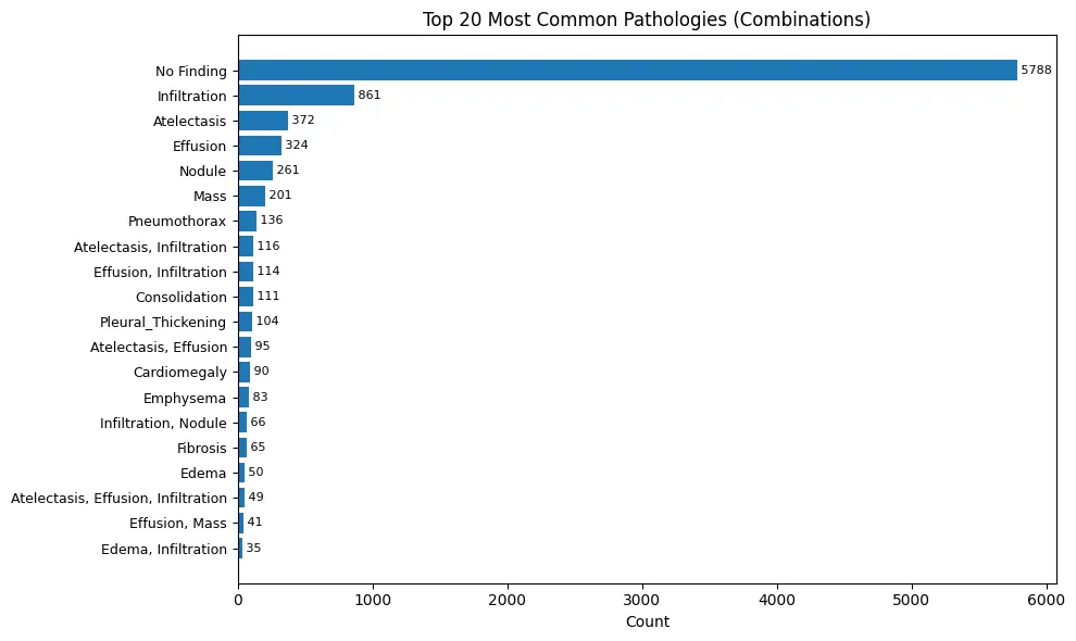
# combinations of labels (pathologies), sorted by occurence
('No Finding', 50500),
('Infiltration', 7327),
('Atelectasis', 3414),
('Effusion', 2788),
('Nodule', 2248),
('Mass', 1696),
('Pneumothorax', 1241),
('Effusion,Infiltration', 991),
('Atelectasis,Infiltration', 981),
('Consolidation', 829),
('Atelectasis,Effusion', 818),
('Pleural_Thickening', 817),
('Cardiomegaly', 777),
('Infiltration,Nodule', 609),
('Emphysema', 587),
('Fibrosis', 551),
# ...

The Naive Approach Fails

A linear classifier to predict the labels simply resorts to predicting “No disease” and still gets away with an accuracy of ~30%.

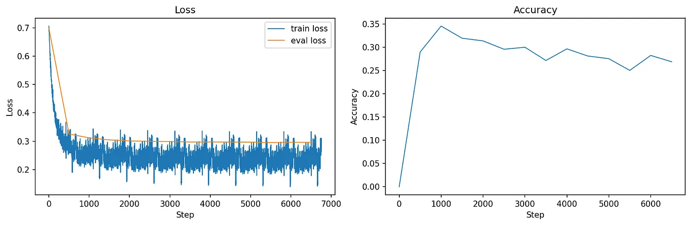
SolveIt suggests weighting the loss, making the loss penalize missed positive predictions more for rare classes.

For example, if “Hernia” appears 100x less often than “No Finding”, you would give it a weight of 100.

That didn’t work either.

Balanced Sampling

We balance the sampling process using a Weighted Sampler and focus on the pathology combinations with at least 500 samples per combo.

# First, filter your dataset
def filter_dataset(ds, min_count=500):
  # Count combinations
  combo_counts = Counter()
  for item in tqdm(ds):
    combo = tuple(sorted(item['labels']))
    combo_counts[combo] += 1
  
  # Keep only combos with >= min_count
  valid_combos = {combo for combo, cnt in combo_counts.items() if cnt >= min_count}
  
  # Filter dataset
  filtered = ds.filter(lambda x: tuple(sorted(x['labels'])) in valid_combos, num_proc=6)
  return filtered, valid_combos

# Then create weights
def get_sample_weights(ds):
  combo_counts = Counter()
  sample_combos = []
  
  for item in tqdm(ds):
    combo = tuple(sorted(item['labels']))
    sample_combos.append(combo)
    combo_counts[combo] += 1
  
  # Weight = 1 / count (so rare combos get higher weight)
  weights = [1.0 / combo_counts[combo] for combo in sample_combos]
  return weights

filtered_ds, valid_combos = filter_dataset(ds["train"], min_count=500)
weights = get_sample_weights(filtered_ds)
sampler = WeightedRandomSampler(weights, num_samples=len(filtered_ds), replacement=True)

dl_train = DataLoader(filtered_ds, batch_size=bs, sampler=sampler, **dl_common_args)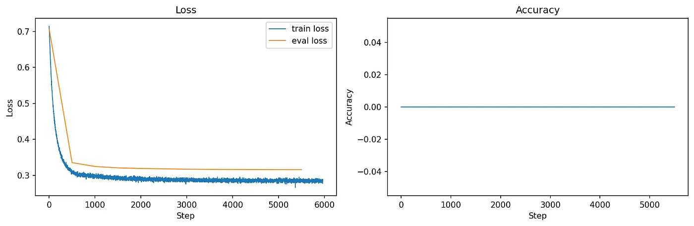

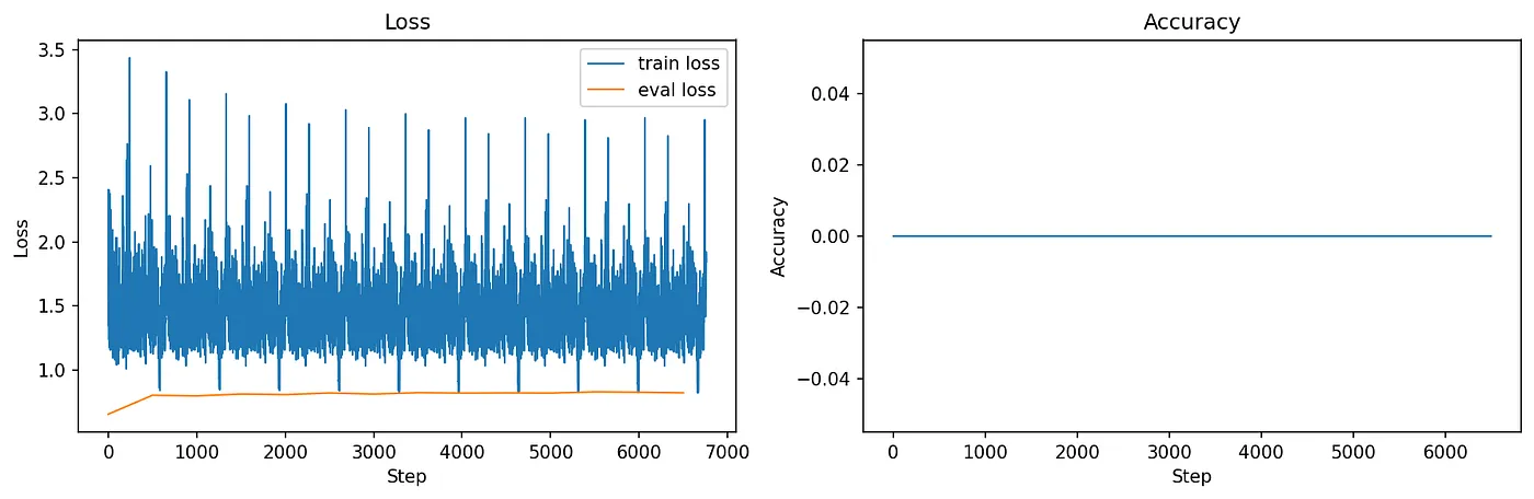
Loss/acc., 10 epochs, batch size 128, LR 0.0001

The classifier learns “something” it seems, the loss goes down continuously. But still accuracy of predictions stays flat at zero.

Train your backbone!

So far we trained a classifier on top of the vision encoder Dino.

Dino outputs a number of embeddings, one for each image patch, and one class token (and a bunch of others). The class token represents the features of the entire image.

For example, the architecture of a Dino-based cat classifier 🐈

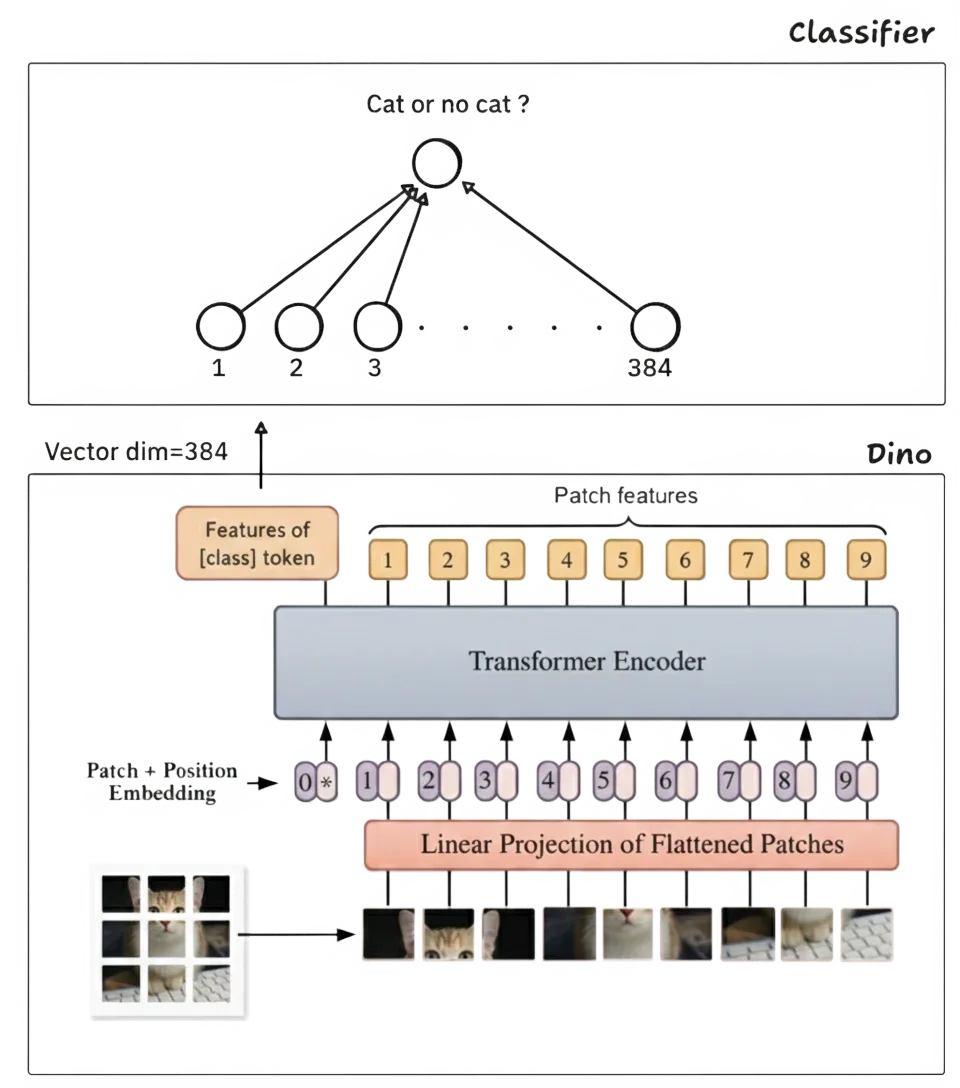
Classifier trained on Dino’s class token. In this case representing something like “a light-furred cat standing on a keyboard.”

Dino trained on 1,689 million images. But maybe it hasn’t seen a lot of X-rays?

If we train the classifier and the Dino backbone ..

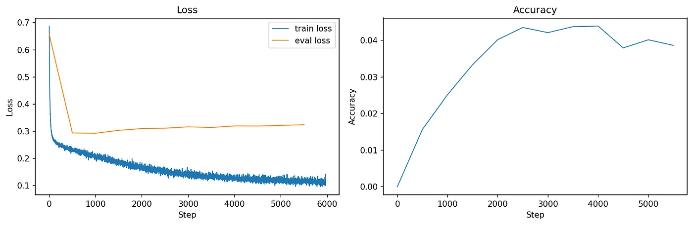
Accuracy >0! Training loss going down, eval loss increasing at some point = overfitting.

Finally a stable descending loss and some accuracy in the predictions! Still, the most common prediction is “No Finding” and the model quickly overfits to the training data.

10 Improvements Later

This is what worked best:

Train classifier and backbone
Balanced Sampling
Train one classifier per pathology
Image augmentations

One Classifier per Pathology

I failed at training a classifier predicting all the pathologies of an image at the same time.

Reality enters. Some pathologies are just harder to predict than others. For humans. What about machines?

I switched to training one classifier per pathology.

def split_by_disease(ds, disease_id, num_proc=2):
    "Split an NIH dataset by disease. Returns idcs of positive and negative items for given disease."
    def has_disease(item, disease_id):
        return dict(has_disease = disease_id in item["labels"])
    ds_split = ds.map(
        partial(has_disease, disease_id=disease_id), 
        num_proc=num_proc, 
        remove_columns=ds.features
    )
    pos_indcs = [idx for idx, item in enumerate(ds_split) if item["has_disease"]]
    neg_indcs = [idx for idx, item in enumerate(ds_split) if not item["has_disease"]]
    return pos_indcs, neg_indcs

def create_weighted_sampler(ds, disease_id, num_proc=2):
    "Create a weighted sampler for a given disease id, will return samples 50% with and 50% without disease"
    pos_indcs, neg_indcs = split_by_disease(ds, disease_id, num_proc=num_proc)
    weights = np.zeros(len(ds))
    weights[pos_indcs] = 1/len(pos_indcs)
    weights[neg_indcs] = 1/len(neg_indcs)

    print(f"create_weighted_sampler() for disease {disease_id}: {len(pos_indcs)}+ve samples ({len(pos_indcs)/len(ds)*100:.2f}%), {len(neg_indcs)}-ve samples")

    sampler = WeightedRandomSampler(weights, num_samples = len(ds))
    
    return sampler

Image Augmentation

To prevent overfitting the images are augmented with random rotation, cropping and more.

Original image (very left) + 4 augmentations.

def augment_img(img, resizeTo=(280, 280)):
    "Augment an xray image by rotating, transforming, changing brightness and color"
    transform = T.Compose([
        T.RandomRotation([-5,5]),
        T.CenterCrop(resizeTo),
        T.RandomResizedCrop(resizeTo, scale=(0.9, 1.0)),
        T.ColorJitter(brightness=0.1, contrast=0.2)
    ])
    return transform(img)

def collate_fn(items, disease_id, img_processor, augment):
    "Turn a list of NIH samples into a batch."
    images = [ i["image"] for i in items ]
    if augment:
        images = [ augment_img(img) for img in images ]        

    images_tensor = torch.stack(
      img_processor(images)["pixel_values"]
    )
    labels_tensor = torch.Tensor([
        (1 if disease_id in i["labels"] else 0) 
        for i in items
    ]).unsqueeze(1) 

    return images_tensor, labels_tensor

Problem Solved?

Some pathologies are indeed harder to spot than others. This applies to biological and artificial neural networks it seems.

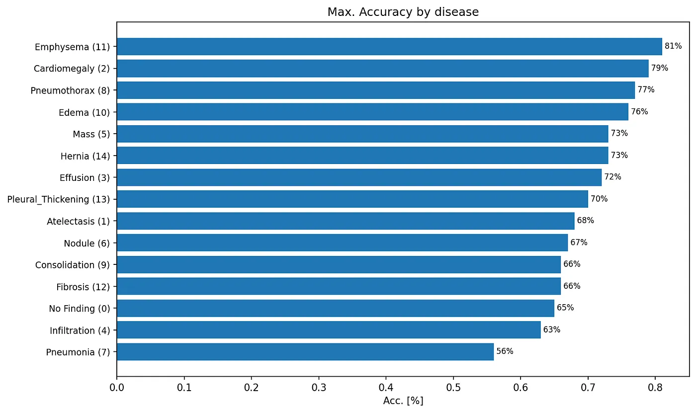
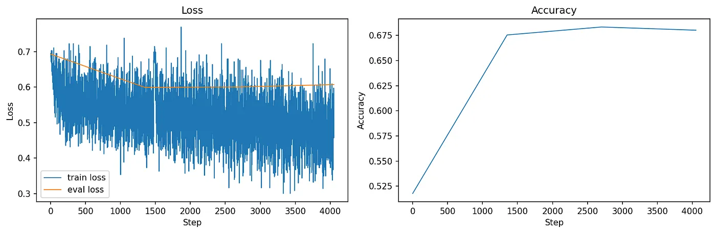
Performance of our neural network in classifying pathologies.

Loss/acc. for “Atelectasis”. There’s still overfitting.

Non-Expert 5 cents: I’m a non-radiologist MD but I have some experience in reading X-rays. I can not 100% relate to the accuracies we see here. Emphysema is hard to me but Pneumonia is fairly easy.

But what did the model actually learn?

Visualizing Attention

“Attention” ? We have to back up for a second. Bear with me please.

You might have heard of it, the attention mechanism sparked a revolution in AI. That’s the thing that led to ChatGPT. Attention is now a popular mechanism used for vision, audio and language models.

Selective Focus

Attention allows tokens to talk to each other.

In vision models like Dino, a token corresponds to an image patch. Let’s take an image of two cats for example. Inside the neural network, attention is a computed matrix of scores 0–1 telling how information flows between tokens.

Let’s see which image patches the class token of Dino attends to.

Left: input. Right: Attention matrix overlay for class token (avg. of all attention heads) of DinoV3. — **Left**: input. **Right**: Attention matrix overlay for class token (avg. of all attention heads) of DinoV3.

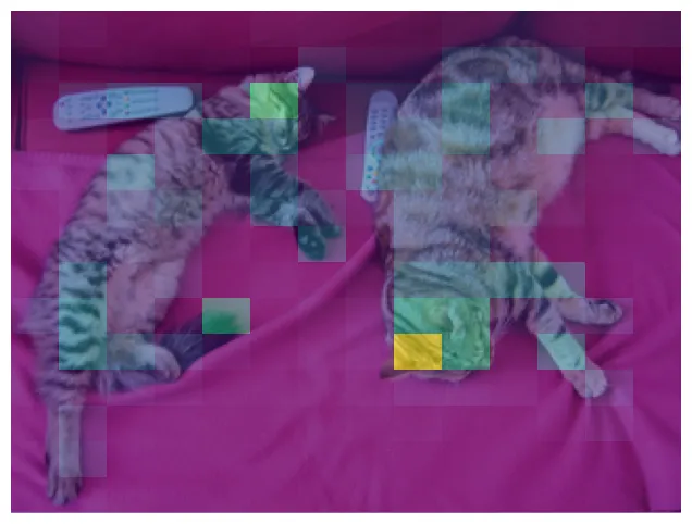
Apparently, Dino thinks the cat bodies and especially the head regions are the important patches in this image.

Back to X-rays.

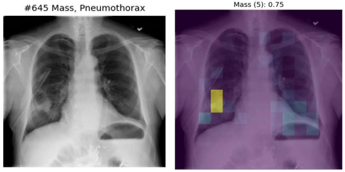
Visualizing the X-Ray Classifier’s Attention

Example of a pulmonary mass X-ray. The classifier we just trained predicts a mass to be present with a probability of 94%.

Left: Input image and labels in the dataset. Right: Attention overlay of model trained to predict “Mass”. — **Left**: Input image and labels in the dataset. **Right**: Attention overlay of model trained to predict “Mass”.

Beautiful, right?

Here’s another one.

Let’s check another pathology, “Cardiomegaly” (big heart).

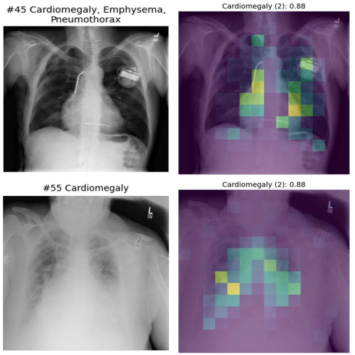
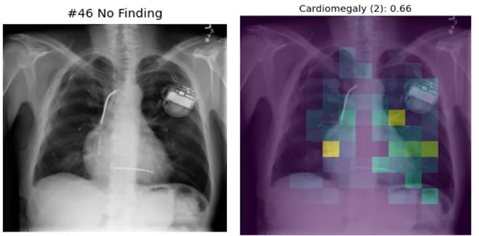
The model focuses on the heart, makes sense. But in the top image it also attends to a device, a pacemaker.

And this is where the problem comes in: Some image features are correlated with each other. Patients with sick hearts more often wear a heart device than others.

“Pseudo”-True Positives

Correct predictions, but probably caused by the wrong feature.

For example, a pneumothorax (air where it should not be) is treated with a chest tube to drain the air. The pneumothorax classifier has therefore learned to focus on the tube to predict the pathology correctly.

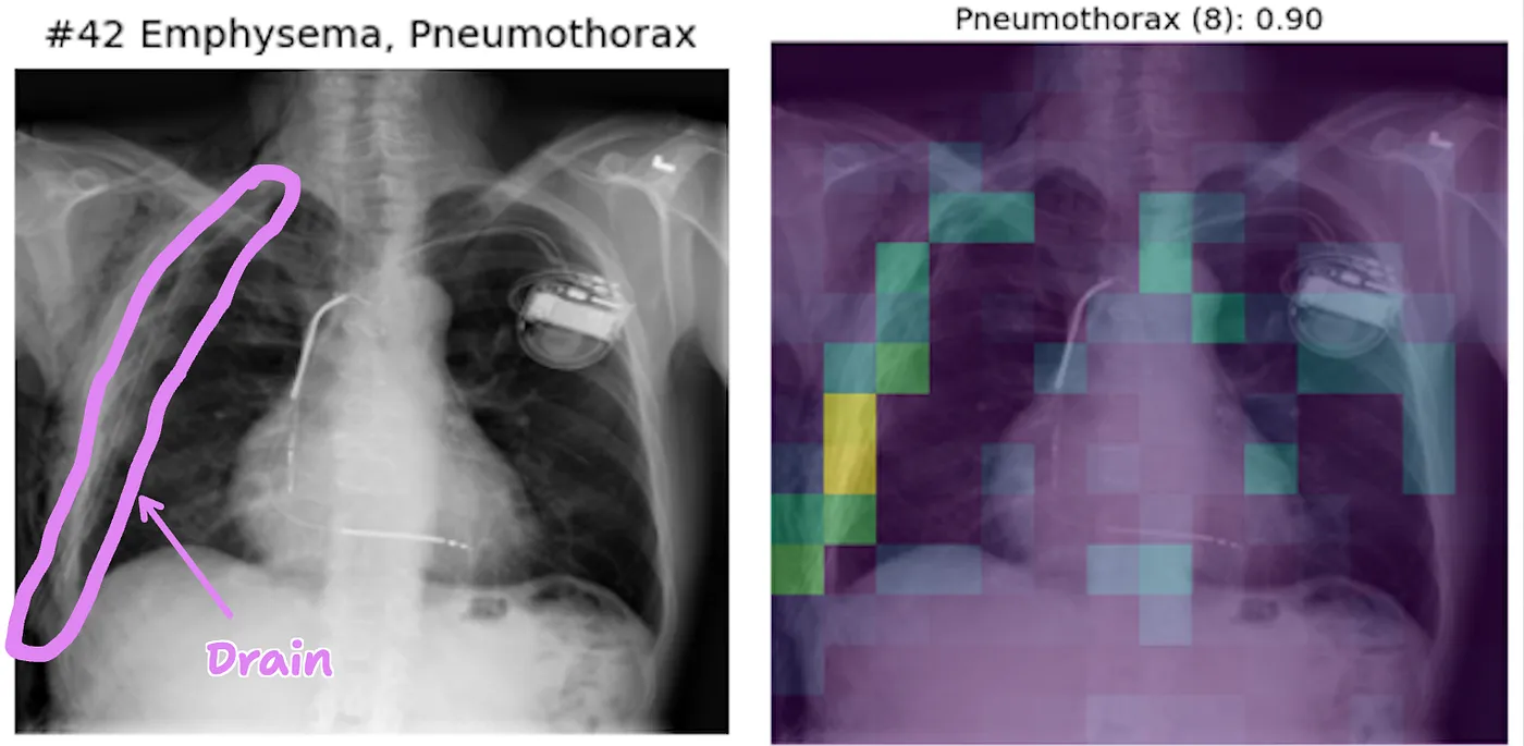
These are all true positives, ie. the model correctly predicts the label.

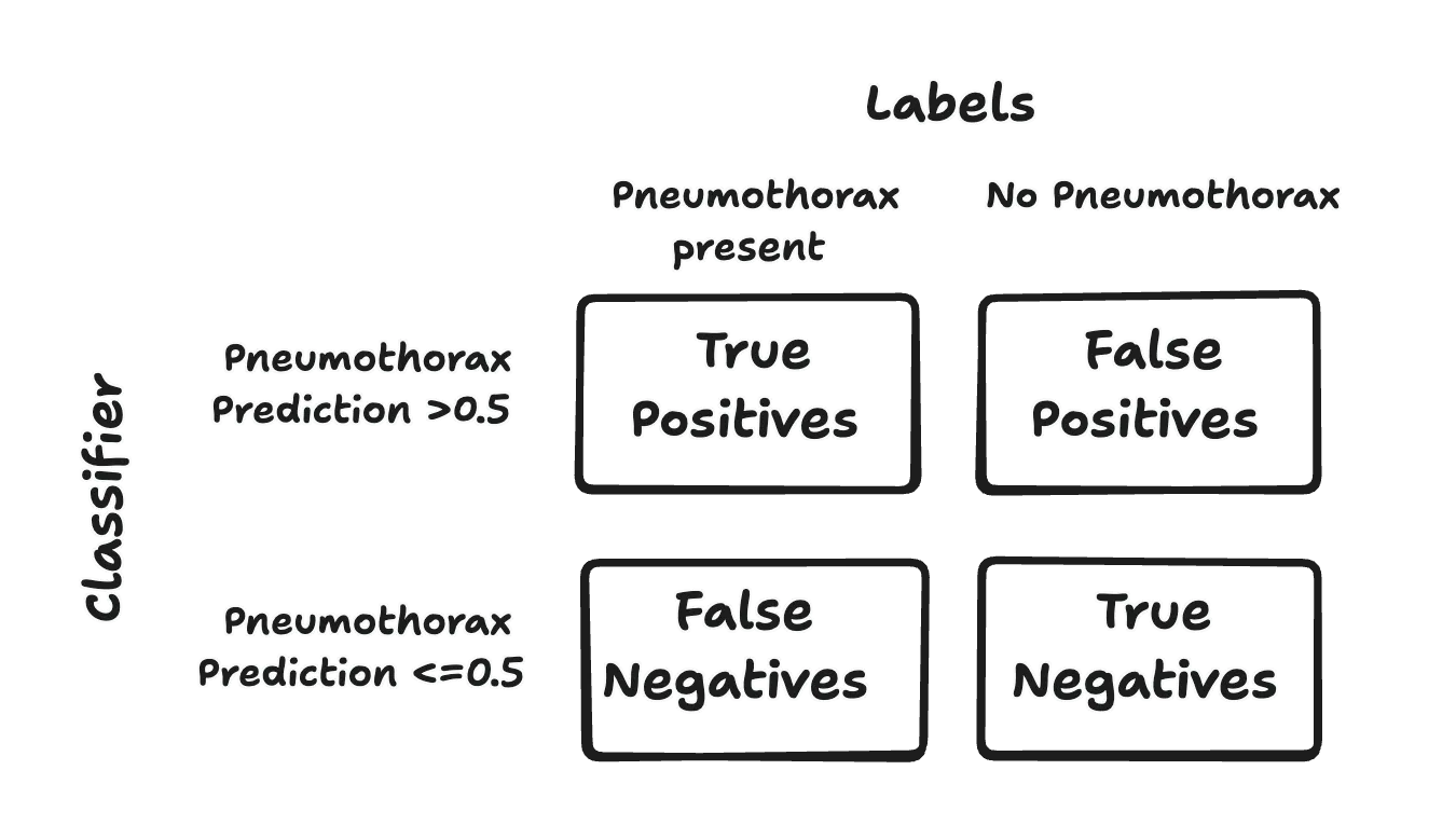
Let’s take a closer look at cases where the model fails.

False Positives

Model predicts a pathology which is not present.

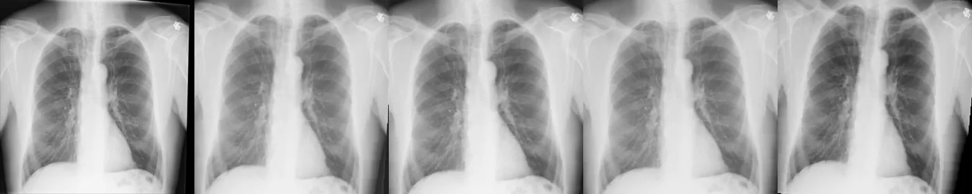
If we look a bit too close at the predictions we could, maybe, also identify problems with data quality.

For example, look at this image #45, labeled as Cardiomegaly (which the classifier predicts correctly).

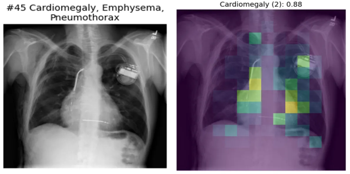
Left: Original image. Right: Classifier prediction and attention visualization. — **Left**: Original image. **Right**: Classifier prediction and attention visualization.

And then image #46 clearly shows the same patient but the x-ray is labeled as “No finding”.

I could go on forever, cherry- and lemon-picking but what’s the point?

Check out the samples of true positives, false positives etc. for all of the classifiers I trained.

This project wasn’t about building the next state-of-the-art X-ray classifier or publishing a scientific paper.

It was a weekend experiment, a chance to tinker, explore, and see what’s possible with a modest setup.

It blows my mind how powerful neural networks are. The model learns to spot pulmonary masses and chest tubes with “just” a bunch (100k) of images and labels. All of that training on a consumer GPU within 10 minutes.

I had fun. Hope you liked it too! Check out the code if you’re interested.